Project Background
A few months ago I was playing Battleship with my daughter. While firing attempting to find her ships by shooting randomly I began to wonder if there was a better way to play the game. That began my search to find a better way. After some research I found the site DataGenetics.
DataGenetics is great site I used to help understand the different methods to search for ships in Battleship. While I implemented the methods demonstrated in my own code I do a slightly different technique after a hit has been registered.
Battleship Basics
As a quick refresher, the rules of Battleship are pretty easy to understand.
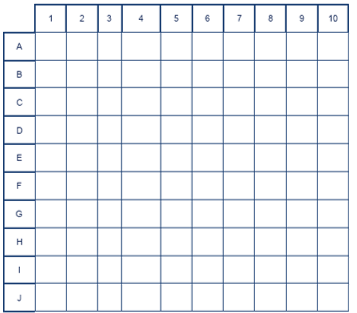
Each player has a 10 x 10 grid to place 5 ships on. The grid is similar to the one below.
Each of the five ships takes up a different footprint on the map.
| Ship Type | Footprint |
|---|---|
| Carrier | 5 |
| Battleship | 4 |
| Submarine | 3 |
| Cruiser | 3 |
| Destroyer | 3 |
Each player will place all ships on their grid. Ship may touch but not overlap.
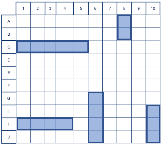
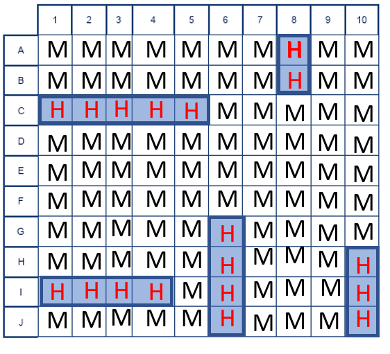
Players will take turns calling our map positions where they think the other player might have placed their ships. The second player will say Hit or Miss, if a hit results in a ship sinking the player will respond with you sunk my “ship name here”. The first player to sink all the enemy ships wins.
An explanation of the different levels
For this project I programed the computer with 5 different levels, from pure random all the way to using a calculation of possibilities to determine the most likely location of enemy ships.
Level 1 - Random
At level 1 the computer will randomly shoot at any space that has not been fired at before. At this level the computer will not pay attention to hits or misses, but will rather just look for empty spots on the board to shoot at. While incredibility inefficient this method will provide a valuable control to assess the future levels at.
Perhaps the key benefit of this level is it is really fast. It the computer will check a dictionary which contains a log of hits and misses and then randomly choose a grid location that has not been shot at. To play a 1000 games in order it takes about 3.4 seconds.
Level 2 - Random With Hunt Mode
This level starts with taking random shots, until the computer hits an enemy ship. When this happens the computer goes into “Hunt Mode”. After the computer registers a hit, it will save the hit location. On the next shot the computer will check the space to the north of the hit. If the space is empty the computer will shoot at that location.

If the space to the north is listed as a miss the computer will check the space to the east of the original hit. Then the south and then the west until there is a Hit.
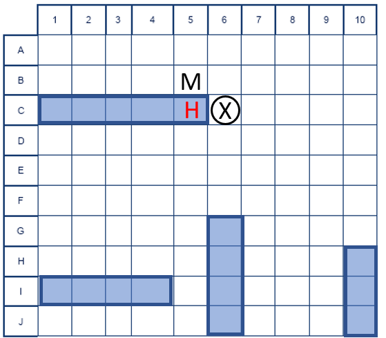
Once a hit is registered the computer will then advance one square in the direction of the hit and shoot at that location. The computer will continue in hunt mode until a ship is sunk.
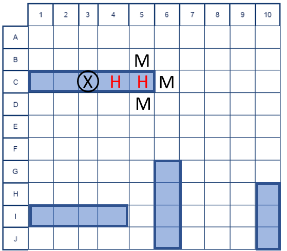
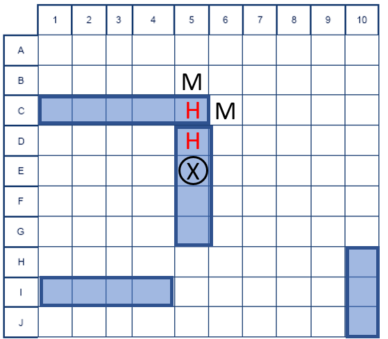
Currently the only problem with hunt mode is it is suspectable to ship stacking, where two ships are placed next to each other. When this happens the computer will follow the path of the second ship until the second ship is sunk. Once the ship is sunk the computer will leave hunt mode with the original ship still afloat.
The level is also fairly fast. For the majority of shots it uses the same method as above to determine the next likely shot. Even when the computer is in “Hunt Mode” it is still just a series of look ups. There is minimal calculations taking place and there for it runs very fast. To play 1000 games in order it takes the computer about 1.98 seconds. As demonstrated in the analysis portion, this reduced time is because the games in level 2 are about 30 moves shorter than games played on level 1.
Level 3 - Parity With Hunt Mode
In parity mode the computer will shoot at every other square. For example the row “A” the computer will shoot at the odd columns (1,3,5,7,9), and on the “B” row the computer will shoot at the even columns (2,4,6,8,10). The computer will choose these locations randomly, and once a hit is scored the computer will enter into “Hunt Mode”.
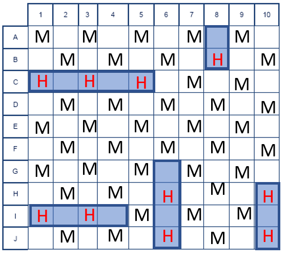
At this point the games are taking longer to be played due to some of the calculations that need to occur. For 1000 games to be played on level 3 it takes 5.4 seconds. The calculations for this level are pretty light, but the cost of calculations is already starting to show.
Level 4 - Probability Mode
Ok first off this is not really a probability but more of a possibility. For each cell of the board the computer will calculate the number of ways a ship can possibly occupy that space. Starting with the Carrier and Cell “A:1”. There are only two ways the Carrier can occupy this cell, so for this cell for the Carrier the value is two.

This process is repeated for each ship type and the number of possibilities is added. So at the start of the game the value of cell “A:1” is 10 and the value of cell “E:5” is 34. As there are more ways to place a ship that will land on E:5 as opposed to A:1, the shot with the best chance of hitting a ship is to shoot at E:5. When there are multiple cells with the same possibility number such as E:5, E:6, F:5, and F:6, the computer will randomly choose one of the highest ranking cells to shoot at.

After each shot the probability board will recalculate. Misses on the board will result in the cell being treated as a zero and will effect the cells around in. For example, this is the board after shooting at E:5 which is a miss.
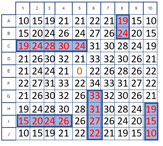
With the ships on the map as shown the computer will need 9 more shots until the first hit at C:3. At this point it is possible to see how even though must of the previous shots were misses, the high numbers are starting to align with the ship locations on the board.
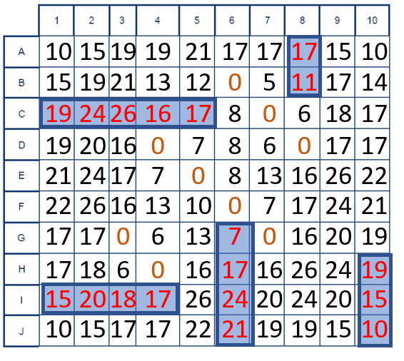
For this level there is no hunt mode as I wanted to see how just going after the most likely locations would effect computer performance. compared to the other modes. At this level the cost of computation becomes clear. As written after each play each cell’s value is calculated for each ship. For a single game this small calculation is not noticeable, but for a 1,000 games to be played there is a definite increase in time. To play 1,000 games it took about 388 seconds which is about 6 minutes. This time could be decreased by implementing multi-threading or parallel processing for the calculations.
Level 5 - Probability With Hunt Mode
This level takes the same approach as level 4 and combines it with the previously mentioned Hunt Mode. This method was able to play 1,000 games in 286 seconds or just over 4 and a half minutes. The reduced time is due to the hunt mode.
Coding the Game
After deciding on the different levels and the types of strategies they would employ, the next step was to actually code the solution. The project was coded in python and used no external libraries. The raw code is located at this github repository CLI-Battleship on GitHub. In order to deploy a solution to test which level performed the best the project was packaged and is listed on PyPi at CLI-Battleship.
The primary focus of this portion of the project was to code the game and the computer levels. However, A single player mode was also constructed. This actually proved to be more time consuming to ensure there was input validation and a easy to read print out of the game board.
Testing Infrastructure Part 1
Now the program was coded, the infrastructure to run the game a million times and save the results needed to be established. Just running each level a single system was not reasonable. To play all games would take an estimated 171,195 seconds or just about 48 hours. This would tie up my machine for a very long time and if there was an error then all that work could potentially be lost. So it was decided to turn the game into a callable API where the results would be saved into a mongoDB.
To accomplish this an API was built using FastAPI and deployed using Kubernetes to orchestrate multiple battleship containers and Rancher to manage the Kubernetes environment. By doing this multiple games of Battleship could be played simultaneously reducing the time required. Each game result would then be stored in a MongoDB for later evaluation. This method was faster than the original method, but still took some time for each level of games to process.
Then disaster struck. The Rancher Cluster and MongoDB database were all self hosted on a local R710, which while old still works very well. Well it did until there was a power surge that fried one of the processors. After the processor was replaced and the cluster rebuilt the process began again. Once all the games had been run and the data was ready for analysis, the database crashed and I was unable to recover it. With the data gone and I was not willing to risk the same amount of time to rebuild the database and potentially lose the data again I decided to move the database to the cloud.
Testing Infrastructure Part 2
There are many cloud providers and many different ways to deploy a database. As I really didn’t want to self install MongoDB on on a linux instance and manage it, I decided to use the managed MongoDB platform offered by Digital Ocean. This was a very easy process to set up an account and the database was ready to populate within 15 minutes. I then reconfigured my FastAPI to send results to the DigitalOcean MongoDB instance.
After a couple of test runs to ensure all the data was moving correctly, I started sending game requests to my local Battleship API. After letting level 1 run I checked the database and noticed several hundred thousand results were missing. It appears that as I was on the cheapest plan I was also being throttled, so not all my results were being allowed to be saved to the database. After some research I decided the fastest option would be to utilize AWS resources.
Testing Infrastructure Part 3
After the issues of trying to use FastAPI to call an instance of the game and then save to MongoDB both local and cloud based, I decided I need the quickest possible way to deploy the solution, run all million games, and visualize the results. This is when I decided to use AWS Lambda to run the million games and save the results to DynamoDB. I was driven to Lambda as I could run all the games concurrently reducing my time for all million games to play from 2 days down to about 5 minutes.
To understand how this is possible it is important to understand AWS Lambda. Lambda acts as “function as a service”, where when the function is called, the function spins up, runs the function, and spins down. As it is serverless, or fully managed by AWS, all I was responsible for was writing the code. When the function was called AWS would handle all the server side functions. This also worked well for my application as each was independent of the next I could in theory run all million games at once, or run all AWS Lambda game functions at once. When working with Lambda it is important to remember that Lambda works best when it is being asked to do exactly one thing that can be accomplished quickly.
The goal was to be able to send a request to Lambda with the computer level and number of games to be played. Then a separate Lambda function would run each game and save the results to DynamoDB. To accomplish this the following architecture was used.

-
API Gateway was connected to a Lambda function, where an API request would save a JSON document in an S3 bucket. The API request would contain the number of games to be played and computer level. This request would be saved as a JSON document in S3.
-
Once the JSON document was placed in S3, another Lambda function would take the JSON document and create a game request in another S3 bucket. For example if 1000 games were requested for computer level 0 was requested, this step would create 1000 JSON documents in the second S3 bucket.
-
For each new JSON document in the S3 bucket a separate Lambda function will be created and the game will be played with the results being saved in DynamoDB.
Visualize and Analyze the Results
With all the games complete and the data saved in DynamoDB it was time to open a Jupyter notebook and start exploring the results.
Level 1 - Random
The results show that just shooting randomly at the board produces shocking bad results. Out of the 250,000 games played for this level the overwhelming majority of games took between 94 and 97 moves to complete. The fastest a game was completed at this level was in 52 moves, and this was only one game. After reviewing these results this is a very poor method in which to play Battleship.
| Number of Moves | Number of Games |
|---|---|
| 97 | 19205 |
| 96 | 19066 |
| 98 | 17852 |
| 95 | 17704 |
| 94 | 16273 |

Level 2 - Random With Hunt Mode
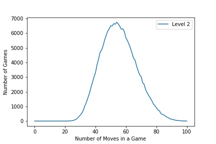
This is method is the method used by most human players. They randomly shoot at the board based on intuition, and when they find a ship they just around the shit until the ship is sunk. This method produced much better results than just randomly shooting, with most games being finished between 51 and 55 moves. The fastest game played at this level was resolved in just 22 moves.
| Number of Moves | Number of Games |
|---|---|
| 54 | 6752 |
| 52 | 6654 |
| 55 | 6635 |
| 53 | 6617 |
| 51 | 6501 |
Level 3 - Parity With Hunt Mode
While not commonly used this method does provide better results than both random and random with hunt modes. While better this mode was only slightly better than the random with hunt mode. Most games were resolved between 49 and 53 moves. Once interesting thing to note is this method produced the fastest game in 19 moves. This means this mode was only 2 games away from a perfect game. While impressive this 19 move game is an anomaly.
| Number of Moves | Number of Games |
|---|---|
| 51 | 9805 |
| 52 | 9718 |
| 53 | 9696 |
| 50 | 9570 |
| 49 | 9392 |

Level 4 - Probability Mode
In this level the computer is shooting at the location where there is most likely a ship, no matter if the last shot was a hit or miss. This method resulted in most games finishing between 56 and 60 moves, with the fastest game being played in 30 moves. This is worse than both the random with hunt and the parity with hunt modes, but will serve as a valuable data point to evaluate the last level.
| Number of Moves | Number of Games |
|---|---|
| 58 | 24955 |
| 57 | 22514 |
| 59 | 21943 |
| 56 | 16948 |
| 60 | 15524 |

Level 5 - Probability With Hunt Mode
In this last level it combines the probability mode with hunt mode for very impressive results. Most games using this method were resolved in 41 to 45 games, with the quickest game being played in 23 moves. This is the most impressive results of any of the game modes.
| Number of Moves | Number of Games |
|---|---|
| 43 | 12086 |
| 42 | 11731 |
| 44 | 11715 |
| 41 | 11132 |
| 45 | 11116 |

Lessons Learned/Final Thoughts
This project started out with a simple question, “What is the most efficient way to play Battleship?” By programming several solutions and deploying them resulted in the graph below after 1,000,000 games of Battleship. Clearly demonstrating the best way to play Battleship is to shoot at the locations where there is most likely to be a ship based on the possible ways a ship can be placed in that square in combination with a hunt mode.

This was one of the more demanding projects I have taken up. It included but was not limited to:
-
Building, packaging, and deploying a Python library to PyPi.
-
Building a deploying FastAPI API using Docker and Kubernetes.
-
Organizing data and saving it in the document store database MongoDB.
-
Deploy API and save results using AWS API Gateway, AWS Lambda, AWS S3, and AWS DynamoDB.
This was a challenging project that required me to pivot my approach to the problem many times. I am glad I stuck with it and worked till I found a solution that was feasible. I have several ideas on how to improve the game level and different approaches. However, I think I am done with this project for now. It has been a great learning experience but it is time to move on to another challenge.
